Modelling
Since it is unknown what kind of spam filter the recipient uses, various machine learning algorithms are compared in terms of their ability to distinguish between spam and non-spam emails. To be able to assess the quality of each model a 5-fold cross-validation procedure is performed. Finally the interpretability of promising algorithms will be analyzed in Interpretable Machine Learning section.
Evaluation Metric
Probably the most straight forward metric to evaluate binary classification tasks is accuracy. Accuracy measures the fraction of correctly classified observations for a specific threshold value (usually 0.5). However, the AUC (area under the ROC curve) measures how true positive rate (recall) and false positive rate trade off and therefore evaluates the classifier for all possible threshold values. Compared to accuracy, AUC is a broader measure that tests the quality of the internal value, which the classifier generates and then compares it to a threshold. Since AUC does not test the quality of a particular choice of threshold, it will be used for the rest of the analysis. In our case, the AUC is equal to the probability that our model ranks a randomly chosen spam mail higher than a randomly chosen non-spam mail.
Interpretable Algorithms
Featureless Model
As we are dealing with a binary classification task, a featureless model will be our very low baseline. As the name suggests, the featureless model takes no features/variables into account and always predicts the most frequent class for all observations. In this dataset, 60% of all emails are non-spam and therefore non-spam is predicted for all observations.
When using the featureless model, it becomes clear why AUC suits this analysis better than accuracy. If always the most frequent class is predicted, the accuracy in our case is 0.6. The AUC however stays at its lowest possible value of 0.5 since the model cannot distinguish between spam and non-spam mails.
Logistic Regression
One algorithm which is inherently interpretable is logistic regression. Here we get a coefficient for each feature and could make statements like “if feature x has a one unit increase the estimated spam probability changes by y, given all other features stay the same (≐ ceteris paribus)”. Realistically, with nearly 60 features and the ceteris paribus assumption the interpretability of a regression model is more than questionable.
Naive Bayes
Another interpretable model is Naive Bayes. In this algorithm, the spam probability is calculated for each observation based on its feature values. With the naive assumption that all features are independent, it is then possible to interpret the conditional probability for each feature and therefore assess each feature's impact on the prediction.
Decision Trees
A single decision tree (cart) allows for very specific statements like “If feature A has value x and feature B has value y class Z will be predicted”. Classification trees have the big advantage of being particularly easy to understand and therefore to interpret. However, such decision rules are quite unstable, oftentimes inaccurate and frequently lead to overfitting. Bagging unstable predictors is suggested (like decision trees) to improve accuracy. Bagging is short for "Bootstrap Aggregating" and is a procedure to average the prediction of multiple predictors to reduce the variance compared to a single predictor. This is the basis for random forests, which will be introduced in detail in the next section.
Non-interpretable Algorithms
Random Forest
The first not easily interpretable model which is considered is random forest. It is an algorithm where multiple decision trees are combined, or aggregated, to improve the single tree’s instability and tendency to overfit. Multiple decision trees are generated, where each tree can only use a subset of features (obtained by bootstrap) for splitting.
However, the straight forward interpretability is lost compared to a single decision tree. For the random forest the parameter mtry in R, which is the number of variables to possibly split at in each node, is tuned prior to the benchmark in a 5-fold cross validation. The AUC optimal value is mtry = 7. By using the data twice, once for hyperparameter tuning and once for the benchmark, we might underestimate the generalization error. However since hyperparameter tuning is computationally expensive, and we are not interested in the precise generalization error of each model but rather the general tendency of each model's performance, we refrained from nested resampling. Additionally, as it has shown in this article, random forests are an efficient way of classifying spam. We will therefore analyze this model class in more detail concerning its interpretability.
Support Vector Machines
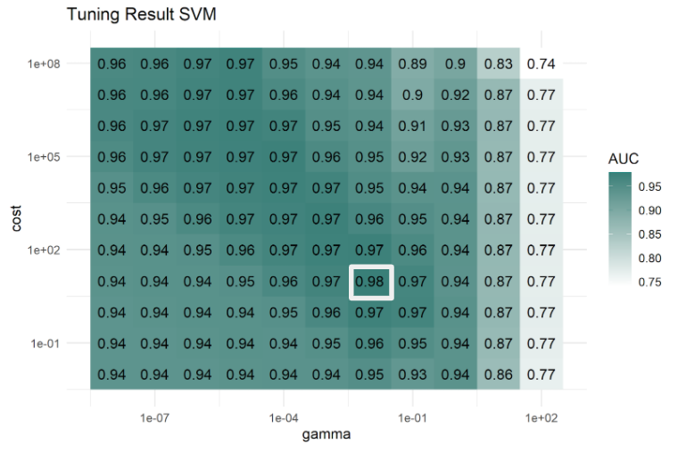
Support vector machines (SVM) try to find a separating hyperplane between the two classes and are not interpretable as well. We refrained from using nested resampling for the same reasons as with random forest. We are not interested in the best possible model, but rather a realistic model, which might be applied in real life by email providers. Thus, in this analysis, a radial kernel will be used and the hyperparameters cost and gamma will be tuned in a 5-fold CV prior to the benchmark. The cost parameter controls how margin violations are penalized. High costs lead to expensive margin violations and therefore to a very narrow margin which in turn might promote overfitting. The parameter gamma from the kernel function k controls the shape of the decision boundary.
A high leads to a wiggly boundary which might also lead to overfitting. As you can see in the image below, both parameters have similar influences on the decision boundary and need to be balanced. As a wide range of combinations of gamma and cost might be suitable, we first tuned on a grid where gamma might take values in , and cost in . A combination close to gamma = 0.01 and cost = 10 was the most promising and therefore a second 5-fold CV was performed for gamma values in [0.001, 0.05] and cost values in [5, 50]. The results of the tuning can be found below. The highest AUC of 0.978 could be achieved with gamma = 0.012 and cost = 13.33. As it has shown in this article, Support Vector Machines (SVM) are a powerful, state-of-the-art method in machine learning to distinguish spam from non-spam. Thus, we will analyze how SVMs obtain their predictions in more detail in Interpretable Machine Learning section.
xGradient Boosting
The last non-interpretable method is xGradient Boosting (xgboost) which uses gradient boosting to build the model. Here the parameters eta, min_child_weight, subsample, colsample_bytree, colsample_bylevel and nrounds will be tuned in a 5-fold CV with grid search. AUC optimal values can be found in Table below.
| Parameter | lower bound | upper bound | AUC optimal value |
|---|---|---|---|
| eta | 0.2 | 0.4 | 0.33 |
| subsample | 0.7 | 0.8 | 0.77 |
| colsample_bytree | 0.9 | 1 | 0.93 |
| colsample_bylevel | 0.5 | 0.7 | 0.5 |
| min_child_weight | 1 | 20 | 1 |
| nrounds | 1 | 200 | 67 |
Benchmarking
The distribution of 5-fold cross-validated AUC values for each model can be found in figure below. There you can also see that models which are inherently not interpretable, like SVM, random forest and xgboost outperformed explainable models like decision trees and logistic regression. It is very likely that email providers use such non-interpretable methods for their spam filters, especially since they are mostly interested in an accurate classification with as little false positives, i.e., emails that are wrongly classified as spam, as possible.
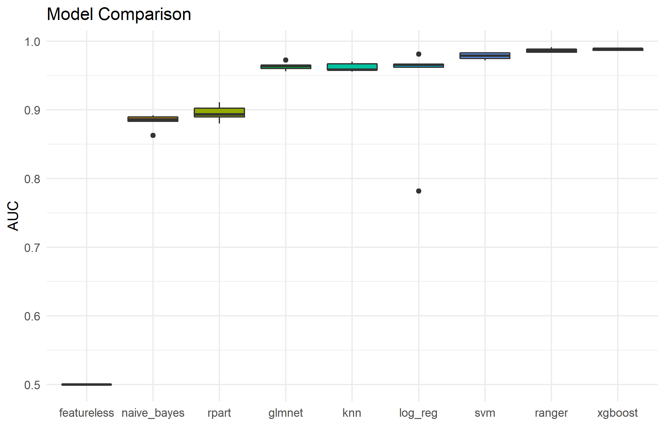
As previous research has shown, random forest and SVM are very well suitable algorithms for spam classification. Since xgboost has a slightly higher false positive rate than random forest as shown in the table below, we will only focus on SVM and random forest in our further analysis of the interpretability of these algorithms. In doing so, a kernel based (SVM) and a tree based (random forest) algorithm will be compared.
| learner | AUC | FPR |
|---|---|---|
| featureless | 0.500 | 0 |
| svm | 0.978 | 0.044 |
| ranger | 0.987 | 0.031 |
| xgboost | 0.988 | 0.032 |
If we now consider the perspective of scammers who want to make sure their emails pass arbitrary spam filters, it is necessary to make the predictions explainable.
Personalization
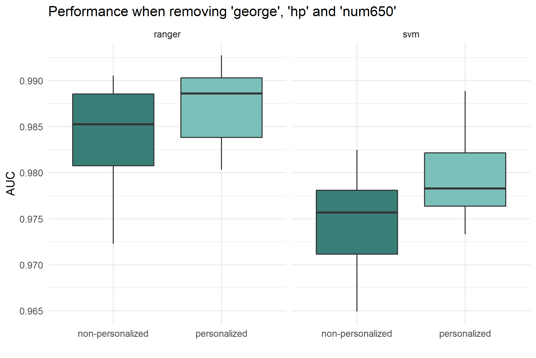
As described in Dataset section, the dataset contains variables on personal information of the recipient, like his name, George, his employer, Hewlett-Packard (HP) and the telephone area code of Palo Alto (650) where the office he works at is located. We are interested in the impact of personal knowledge on the classification. More precisely, we want to assess in what way the personalized features impact the prediction. A separate hyperparameter tuning procedure was performed for the non-personalized dataset, and the same parameters were found to be AUC-optimal. This is the reason the same hyperparameters are used for modeling spam probability with non-personalized features as for the personalized dataset.
In the figure below, it can be seen that both SVM and Random Forest gain AUC when the personalized features are included. This is plausible, as knowing the name or workplace of the recipient is a strong indication that this email is from a known sender and not anonymous spam.